Your first project

You’ll need Flux installed. The plotting step uses Python and fluxplot; you can also begin with an SVG or PNG you already have. All numbers in the small example below are synthetic.

Shortcuts are written with Ctrl and Alt. On macOS, press ⌘ Command for Ctrl and ⌥ Option for Alt; Keyboard shortcuts lists them all.

1. Give the work a home#

Create a working folder called growth-study. In Flux, choose New project from Home and create a project named paper inside that folder.

growth-study/
└── paper/         ← your Flux project

Your analysis code will live in growth-study; the project holds the writing, plots, figures, references, and slides. Flux autosaves your work. If saving reports an error, resolve it before closing the app.

You can return to the project from Home, or open it from a terminal:

flux /path/to/growth-study/paper

Learn how projects and files fit together.

2. Make a plot with named parts#

In a terminal, move to growth-study and create a Python environment:

uv init
uv add fluxplot

Save the following as make_growth.py beside the paper folder. You use ordinary matplotlib axes; fluxplot adds a stable name to each series and saves the semantic files.

from pathlib import Path
import matplotlib
matplotlib.use("Agg")
import matplotlib.pyplot as plt
import fluxplot as fp

time = [0, 4, 8, 12, 16, 20, 24]
control = [0.02, 0.05, 0.13, 0.41,
           0.95, 1.60, 1.90]
treatment = [0.02, 0.07, 0.25, 0.80,
             1.50, 1.95, 2.10]

fig, ax = plt.subplots(figsize=(4.8, 3.2))
fp.line(ax, time, control,
        series="control",
        marker="o", label="Control")
fp.line(ax, time, treatment,
        series="treatment",
        marker="s", label="Treatment")
ax.set(xlabel="Time (h)",
       ylabel="Illustrative response")
ax.set_title("Synthetic growth profiles")
ax.legend(frameon=False)
fig.tight_layout()

here = Path(__file__).resolve()
plots = here.parent / "paper" / "plots"
plots.mkdir(parents=True, exist_ok=True)
recipe = {"script": str(here),
          "params": {}, "inputs": []}
fp.save(fig, plots / "growth.svg",
        recipe=recipe)

Run it:

uv run python make_growth.py

You now have three neighboring files in paper/plots/: growth.svg, growth.fluxplot.json, and growth.recipe.json. Keep them together. The SVG is the visible plot; the manifest describes its parts and data; the recipe records its producing script.

3. Compose and refine in Figure#

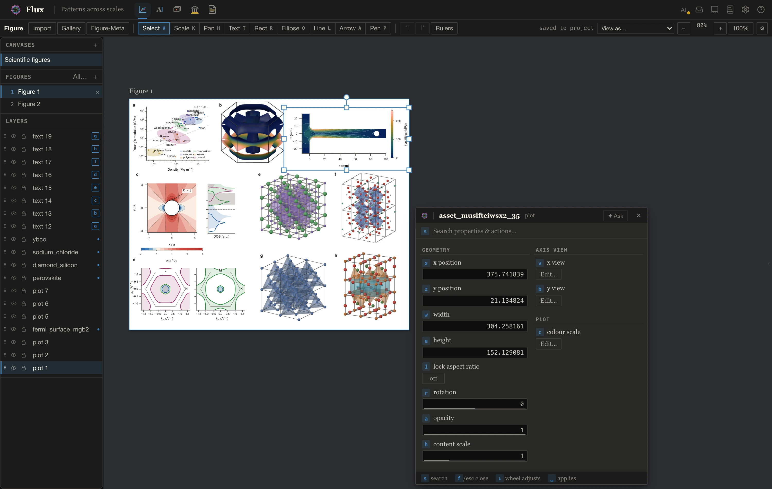
Switch to Figure in the titlebar. Open the Plot gallery with Alt+G, select growth.svg, and choose Insert. Flux imports at the plot’s physical size; the gallery marks semantic plots with a ◆ badge.

Select a plot part with Ctrl+click. Press F to open its properties and change a line’s stroke colour. Alt+R opens X-ray, where you can inspect the plot’s named parts and regeneration recipe.

Try changing a number in make_growth.py and rerunning it. Flux refreshes the linked plot, retaining styling attached to stable series identities such as control. Source status in the figure catalog tells you whether the link is current, missing, or needs attention.

Open Figure-Meta with Alt+M and add a caption. For this example: “Synthetic growth profiles for two illustrative conditions. Points show constructed values at seven time points; lines connect successive observations.”

4. Collect and read a reference#

Open Library and paste a paper’s DOI into the add field, or import a BibTeX file. The reference joins your shared library, where it is available across projects. Use Enrich for additional metadata and the download control for an available open-access PDF.

Open the paper in Reader from its Library row. Select a sentence and choose a highlight colour, then attach a note to the highlight. Reader also supports tabs, side-by-side reading, and figure snips that retain their source provenance.

A reference in your Library becomes part of a project’s bibliography when you cite it. Library and project references explains the distinction.

5. Write with the figure in view#

Switch to Paper and write a short paragraph. Three insertions connect the document to your work:

• Type /figure and choose your figure to embed it with its caption.
• Type @@ to insert a cross-reference to the figure in your prose.
• Type @ and an author’s name to choose a citation from your library.

Figure numbering follows the designation you choose in Figure. Reordering paragraphs does not renumber your figures. The permanent reference stays attached when you rename a figure or move it between canvases.

Your manuscript remains a .qmd file. You can write equations, add tables, keep working notes, and review comments alongside the prose.

6. Let the explanation unfold#

In Slides, compose a slide from the same plot sources. Add a beat for the next part of your explanation, then use the animation tools to reveal an element or transform it into a later state. Present at your own pace.

An interactive slide can also live inside a Paper document. HTML preserves its steps; PDF and Word use a still. The example below runs in Flux’s native player. These are the slides from the Flux film, made from plots in the demonstration project.

Play the slidesThe slides from the film, running in your browser

The example opens on the slide made live in the film: the dots of a plotted Flux mark become five shapes and a caption. Use the arrows to advance, or choose another slide from the menu. Each slide names its data source below the player. Visual credits · Slides guide.

7. Export and keep the sources#

In Paper, choose Export and select PDF. Flux’s built-in PDF export does not require Quarto. Word export uses Quarto; install it through Set up Flux if needed. The command-line route, flux compile --to pdf, uses Quarto and also needs TeX (PDF dependencies).

Check the exported figures, captions, and references, then keep your project folder alongside the result. It contains the editable work you will want for the next revision.